── Attaching core tidyverse packages ──────────────────────── tidyverse 2.0.0 ──
✔ dplyr     1.1.4     ✔ readr     2.1.5
✔ forcats   1.0.0     ✔ stringr   1.5.1
✔ ggplot2   3.5.1     ✔ tibble    3.2.1
✔ lubridate 1.9.3     ✔ tidyr     1.3.1
✔ purrr     1.0.2
── Conflicts ────────────────────────────────────────── tidyverse_conflicts() ──
✖ dplyr::filter() masks stats::filter()
✖ dplyr::lag()    masks stats::lag()
ℹ Use the conflicted package (<http://conflicted.r-lib.org/>) to force all conflicts to become errors
library(ggformula) # Formula based plots
Loading required package: scales

Attaching package: 'scales'

The following object is masked from 'package:purrr':

    discard

The following object is masked from 'package:readr':

    col_factor

Loading required package: ggridges

New to ggformula?  Try the tutorials:
    learnr::run_tutorial("introduction", package = "ggformula")
    learnr::run_tutorial("refining", package = "ggformula")
library(mosaic) # Data inspection and Statistical Inference
Registered S3 method overwritten by 'mosaic':
  method                           from
  fortify.SpatialPolygonsDataFrame ggplot2

The 'mosaic' package masks several functions from core packages in order to add
additional features.  The original behavior of these functions should not be affected by this.

Attaching package: 'mosaic'

The following object is masked from 'package:Matrix':

    mean

The following object is masked from 'package:scales':

    rescale

The following objects are masked from 'package:dplyr':

    count, do, tally

The following object is masked from 'package:purrr':

    cross

The following object is masked from 'package:ggplot2':

    stat

The following objects are masked from 'package:stats':

    binom.test, cor, cor.test, cov, fivenum, IQR, median, prop.test,
    quantile, sd, t.test, var

The following objects are masked from 'package:base':

    max, mean, min, prod, range, sample, sum
Attaching package: 'supernova'

The following object is masked from 'package:scales':

    number
frogs_orig <-read_csv("../../data/frogs.csv")
Rows: 60 Columns: 4
── Column specification ────────────────────────────────────────────────────────
Delimiter: ","
dbl (4): Frogspawn sample id, Temperature13, Temperature18, Temperature25

ℹ Use `spec()` to retrieve the full column specification for this data.
ℹ Specify the column types or set `show_col_types = FALSE` to quiet this message.
frogs_orig
# A tibble: 60 × 4
   `Frogspawn sample id` Temperature13 Temperature18 Temperature25
                   <dbl>         <dbl>         <dbl>         <dbl>
 1                     1            24            NA            NA
 2                     2            NA            21            NA
 3                     3            NA            NA            18
 4                     4            26            NA            NA
 5                     5            NA            22            NA
 6                     6            NA            NA            14
 7                     7            27            NA            NA
 8                     8            NA            22            NA
 9                     9            NA            NA            15
10                    10            27            NA            NA
# ℹ 50 more rows
inspect(frogs_orig)
quantitative variables:
                 name   class min    Q1 median    Q3 max mean        sd  n
1 Frogspawn sample id numeric   1 15.75   30.5 45.25  60 30.5 17.464249 60
2       Temperature13 numeric  24 26.00   26.5 27.00  28 26.3  1.128576 20
3       Temperature18 numeric  19 20.00   21.0 22.00  23 21.0  1.123903 20
4       Temperature25 numeric  14 15.00   16.5 17.00  18 16.2  1.196486 20
  missing
1       0
2      40
3      40
4      40
frogs_orig %>%pivot_longer( .,cols =starts_with("Temperature"),cols_vary ="fastest",# new in pivot_longernames_to ="Temp",values_to ="Time" ) %>%drop_na() %>%##separate_wider_regex(cols = Temp,# knock off the unnecessary "Temperature" word# Just keep the digits thereafterpatterns =c("Temperature", TempFac ="\\d+"),cols_remove =TRUE ) %>%# Convert Temp into TempFac, a 3-level factormutate(TempFac =factor(x = TempFac,levels =c(13, 18, 25),labels =c("13", "18", "25") )) %>%rename("Id"=`Frogspawn sample id`) -> frogs_longfrogs_long
# A tibble: 3 × 2
  TempFac     n
  <fct>   <int>
1 13         20
2 18         20
3 25         20
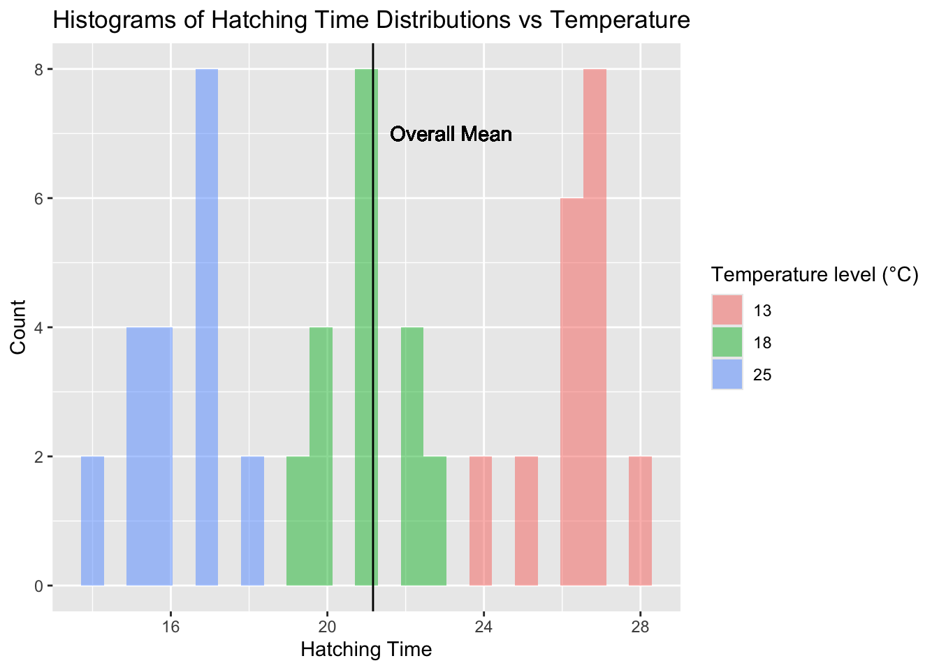
gf_histogram(~Time,fill =~TempFac,data = frogs_long, alpha =0.5) %>%gf_vline(xintercept =~mean(Time)) %>%gf_labs(title ="Histograms of Hatching Time Distributions vs Temperature",x ="Hatching Time", y ="Count" ) %>%gf_text(7~ (mean(Time) +2),label ="Overall Mean" ) %>%gf_refine(guides(fill =guide_legend(title ="Temperature level (°C)")))
gf_boxplot(data = frogs_long, Time ~ TempFac,fill =~TempFac,alpha =0.5) %>%gf_vline(xintercept =~mean(Time)) %>%gf_labs(title ="Boxplots of Hatching Time Distributions vs Temperature",x ="Temperature", y ="Hatching Time",caption ="Using ggprism" ) %>%gf_refine(scale_x_discrete(guide ="prism_bracket"),guides(fill =guide_legend(title ="Temperature level (°C)")) )
Warning: The S3 guide system was deprecated in ggplot2 3.5.0.
ℹ It has been replaced by a ggproto system that can be extended.
ANOVA
frogs_anova <-aov(Time ~ TempFac, data = frogs_long)frogs_anova
Call:
   aov(formula = Time ~ TempFac, data = frogs_long)

Terms:
                 TempFac Residuals
Sum of Squares  1020.933    75.400
Deg. of Freedom        2        57

Residual standard error: 1.150133
Estimated effects may be unbalanced